Supported Geometry Types
GEOS BI supports a variety of geometry types
GEOS BI offers robust support for multiple geometry types, such as circles, lines, and polygons.
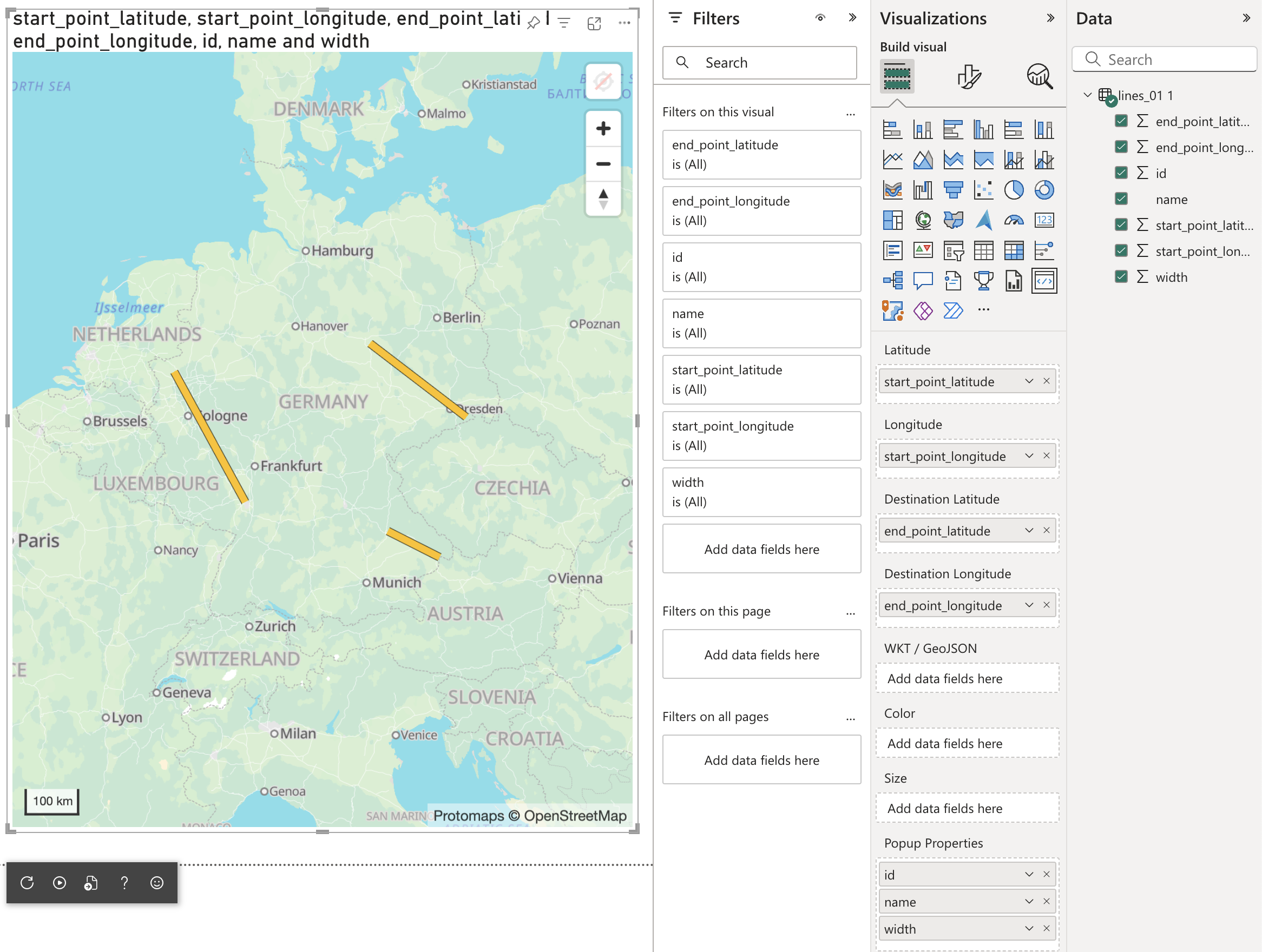
Lines (Defined by two coordinates)
To demonstrate the use of line geometries, we’ll use the following dataset:
| id | name | width | start_point_latitude | start_point_longitude | end_point_latitude | end_point_longitude |
|---|---|---|---|---|---|---|
| 1 | Rhine River Segment | 500 | 51.652249 | 6.6003785 | 49.512211 | 8.4361953 |
| 2 | Elbe River Segment | 700 | 52.104592 | 11.662477 | 50.916128 | 14.152070 |
| 3 | Danube River Segment | 1000 | 48.577033 | 13.460849 | 49.021126 | 12.123448 |
You can download the dataset here: lines_01.csv
To visualize lines on the map, simply put the four location columns (start and end coordinates) into the first four data fields of the visual. The result will look like this:
Multi-LineStrings, Polygons and other complex geometries
You've added a WKT or GeoJSON source, but nothing appears on the map?
One common reason is that the geometry data is too detailed and exceeds Power BI’s character limit (32,767 characters per cell). This means that if any geometry string (for example, a WKT or GeoJSON feature) in a single field exceeds 32,767 characters, Power BI will not display any rows for that visual — even if all other rows are valid. This limit applies to each individual cell in your dataset, not the total file size.
Here’s how you can avoid this issue:
-
Reduce precision: Coordinates are often stored with a lot of decimal places, which is usually more detail than needed and makes the data longer. Rounding to 4 decimal places is accurate enough for most cases. In QGIS, you can do this efficiently with the ‘Snap to Grid’ tool in the processing toolbox.
Example:
The second version is much shorter and still accurate for most mapping purposes.
-
Simplify the layer: If your shapes are generated by an algorithm (like catchment or river delineation), they may contain far more points than necessary, resulting in large data files. Simplifying the shapes can help, though it may slightly affect boundary accuracy.
-
Use single geometries instead of multi-geometries: Instead of using MultiLineString or MultiPolygon, use individual LineString or Polygon geometries. If a LineString is too large, you can split it into several LineStrings and place each in a separate column. This reduces the size of each geometry and helps avoid character limits.
For more complex geometries, such as Multi-LineStrings or Polygons, GEOS BI supports industry-standard formats like GeoJSON and WKT (Well-Known Text).
To use these formats, place the GeoJSON or WKT data into the designated WKT/GeoJSON data field.
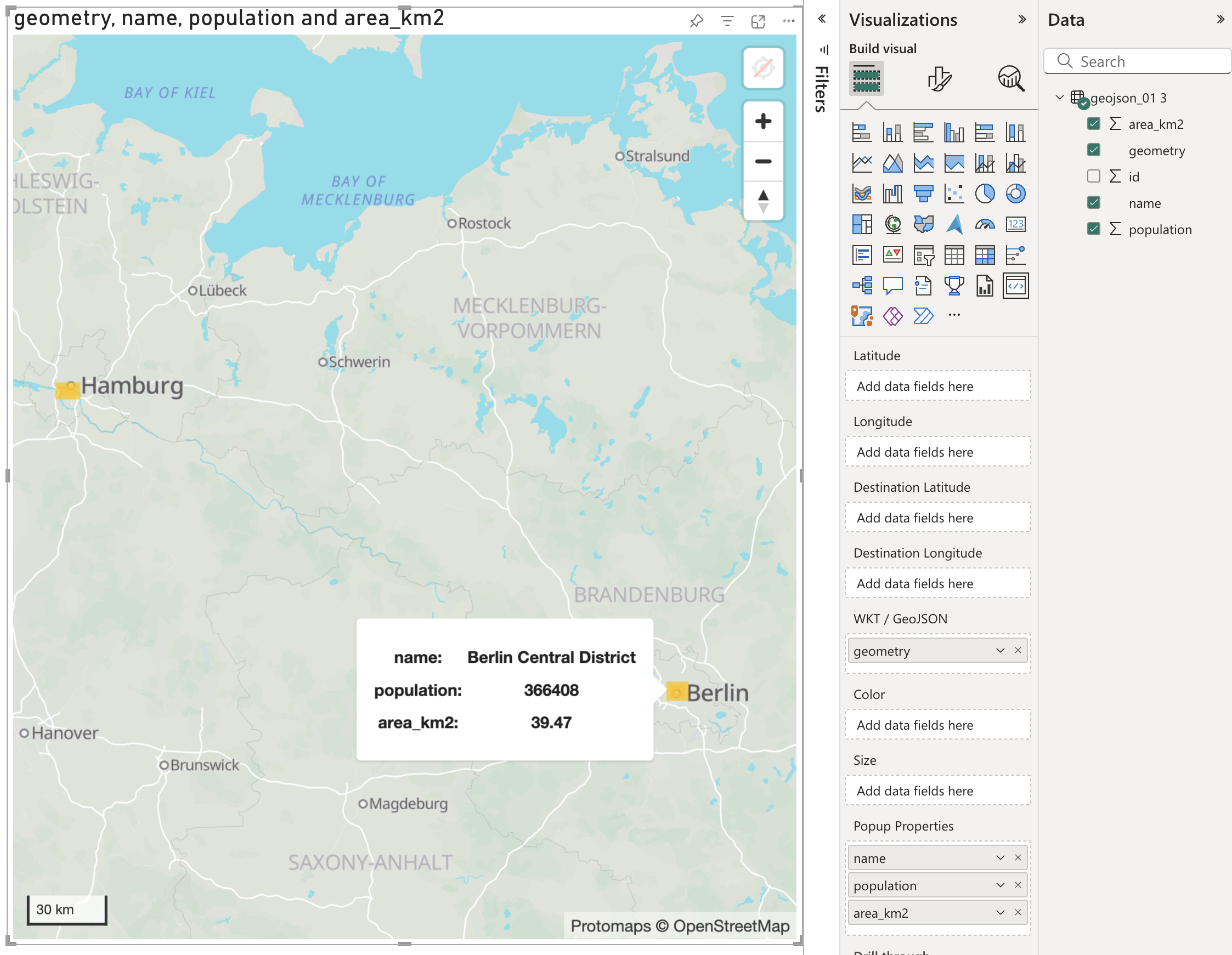
GeoJSON
Here’s a sample dataset using GeoJSON:
| id | name | area_km2 | population | geometry |
|---|---|---|---|---|
| 1 | Berlin Central District | 39.47 | 366408 | {"type": "Feature", "properties": {}, "geometry": {"type": "Polygon", "coordinates": [[[13.366,52.537],[13.366,52.500],[13.445,52.500],[13.445,52.537],[13.366,52.537]]]}} |
| 2 | Munich Old Town | 310.43 | 1488206 | {"type": "Feature", "properties": {}, "geometry": {"type": "Polygon", "coordinates": [[[11.565,48.146],[11.565,48.129],[11.589,48.129],[11.589,48.146],[11.565,48.146]]]}} |
| 3 | Hamburg Harbor | 755.22 | 1841179 | {"type": "Feature", "properties": {}, "geometry": {"type": "Polygon", "coordinates": [[[9.936,53.548],[9.936,53.518],[10.030,53.518],[10.030,53.548],[9.936,53.548]]]}} |
Download the dataset here: geojson_01.csv
When visualized in Power BI, the data appears as follows:
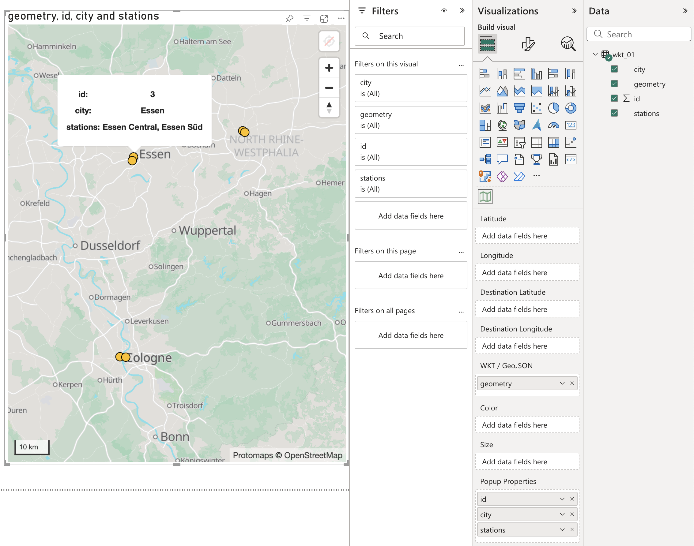
WKT
For WKT-formatted data, here’s an example dataset:
| id | city | stations | geometry |
|---|---|---|---|
| 1 | Cologne | Cologne Central, Cologne Messe/Deutz | MULTIPOINT ((6.958307 50.941357), (6.982230 50.940326)) |
| 2 | Dortmund | Dortmund Central, Dortmund Stadthaus | MULTIPOINT ((7.458076 51.517781), (7.466944 51.514167)) |
| 3 | Essen | Essen Central, Essen Süd | MULTIPOINT ((7.013750 51.451389), (7.008611 51.441944)) |
You can download the dataset here: wkt_01.csv
In Power BI, the WKT data is visualized as shown below: